Simulating Diminishing Returns
“How high is up?”
One of the most important outcomes when measuring ROI for a marketing campaign, is the ability to predict how the ROI could change as adjustments are made to the campaign’s execution. If the ROI is strong, it would be reasonable to conclude that we should increase our spending, but we know from common sense that we can’t just continue increasing spending forever, the ROI will eventually go down.
This is a trap that many marketing teams fall into when they see great results from a new campaign and immediately scale up investment without considering the fact that a consumer’s ninth and tenth exposure to an ad won’t deliver the same impact as the second and third.
Using advanced statistics and quadratic transformations, we are able to replicate real-life diminishing returns impacts in the context of a linear model. As we can do with Adstock and retentions, where the residual impact of an advertisement can remain with a consumer for weeks after exposure, so too can we run an iterative test of different diminishing returns transformations on our target variable (in this case TV GRPs) to tease out diminishing returns rates. One drawback to this method, however, is there are infinite parameters and transformations to test. Therefore, we must be able to reduce the number of potential outcomes to a manageable set that our simulation (and analyst) can reasonably explain.
This tool is designed to provide a visual representation of different iterations of the diminishing returns function. There are parameters that the modeler can adjust for the retention rate (Adstock) and the two constants in the quadratic equation. By adjusting the sliders at the top left, the modeler can familiarize herself with all the potential outcomes of her modeling test and easily eliminate iterations that are impossible.
On the left side, we see the weekly activity levels for our simulated TV campaign. As we adjust the parameters, the Adstock and Saturation curves adjust accordingly. The red line is a visual representation of the variable that is being tested in our model. As weekly weights increase, the relative amount of activity will stretch or compress based on the transformation which is our mathematical representation of real-life diminishing returns.
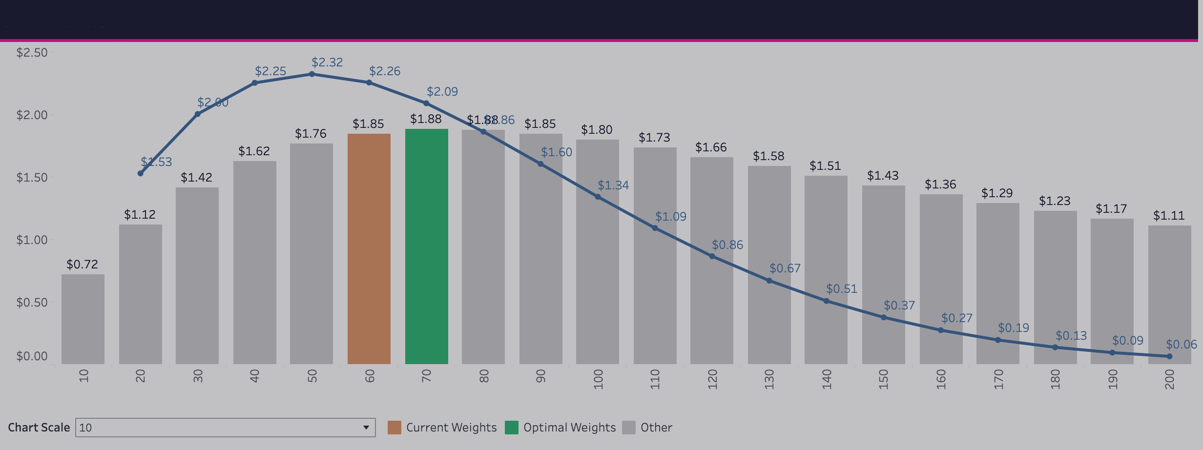
On the right side, we see the ROI and Marginal ROI outcomes at progressively higher weekly activity levels. For our simulated example, our brand achieved an ROI of $1.86 on $14MM in spending behind a two-year flight of 5,353 TV GRPs. Depending on the function parameters, ROI may go up or down as weekly activity increases. We can see for example, what our ROI would be if we executed 100 GRPs per week instead of the current 65 GRPs per week.
The blue line represents Marginal ROI, or the return on investment on the next dollar spent. When Marginal ROI dips below $1.00, then our investment is no longer profitable, and when it drops to $0.00, we’re burning cash. (Gross oversimplification here, but it’s a good benchmark for performance)
An important note about this tool is that it does NOT do all of the work. Because of the dramatic range in outcomes, a statistical modeling exercise must be conducted to determine the parameters that deliver the best fit. After the test is conducted and validated, these parameters can be input in a simulation tool incorporating other media channels to make a determination on how much our brand should increase or decrease TV spending in order to maximize ROI.

